en English
Untitled English subtitles
Report a problem
Advertisement
English transcript
Welcome to the second class of this non-linear vibration of module 3. So, in this class we
will continue, the solution procedure of the non-linear equations; and in the previous
class, we have reviewed or we know about, what is a solution or equilibrium points,
types of equilibrium points, representation of the solution, and how solution of a linear
and non-linear systems differ? And how to determine the solution? So, in the last class
I told you, to determine this solution, so we can apply or we can go for a qualitative
analysis or we can have this quantitative analysis.
So, in case of the qualitative analysis, we have seen how to plot the phase portrait to
find the response of the system? And also to find the equilibrium points, let us take
few examples: few more examples and let us see, how to how these equilibrium points are
determined?
For example, so let us take this example: Let, we have a equation x double dot plus
x minus 0.1 x cube equal to 0. So, as told before in case of the equilibrium position,
or in case of the equilibrium solution, so if it is steady state solution, then it will
not be a function of time. So, this x double dot or any function of any variation of x,
with time should be neglected, so in this case, we can neglect this x double dot equal
to put x double dot equal to 0.
And the remaining thing, we can write as x minus 0.1 x cube equal to 0; and this will
give rise to x into 1 minus 0.1 x square equal to 0 or so, in this case we can have this
x either x equal to 0 or, this 1 minus 0.1 x square equal to 0, which will give rise
to x square equal to 10 or x equal to plus minus 3.1627. So, in this case, we have 3
values of this x so, these 3 are the equilibrium position for this equation.
So in this equation, x equal to 0 refers to the trivial solution, and x equal to plus
minus this 3.1627 are the non trivial solution of the system. So, one can use this qualitative
analysis procedure, to find the phase portrait of this equation, and one can check, whether
these points correspond to this center saddle point? and one can find the separate ricks
also in this case? So, let us take another example: So in this case, let us take this
equation. In this form, x double dot minus x plus 0.1 x cube equal to 0. So, in the previous
case, the this is similar to, this doffing equation with a subtending type of spring
with cubic nonlinearity. This is we have this minus 0.1 x cube.
And in this case, we have taken a equation, we have this linear stiffness part is written
as negative. So, in this case for this steady state solution, this x double dot will be
equal to 0, and this equation can be written as so x minus 0.1 x cube equal to 0. So, we
can have the solution x or x into 1 minus, so x into 1 minus 0.1 x square equal to 0
or, we can have x equal to 0 and x equal to plus minus 3.1627. So in this case also, we
have same solution; that is x equal to 0 is a solution and x equal to plus minus 3.1627
another two solutions; so these are the equilibrium points of this equation.
So, let us take another example; so in this case; so let us take the example; example
3: So, in this case u double dot plus omega 0 square u equal to epsilon into u dot minus,
let me take this u dot u cube. So, in this case for steady state, one can put this u
dot and u double equal to 0. So by putting, u dot and u double dot equal to 0. So, one
can obtain the equilibrium solution as omega 0 square u equal to 0 or u equal to 0. So,
this u equal to 0 represents the equilibrium solution in this case.
So, one can obtain; so this is the 100 pole equation, and the previous two equations are
doffing equations. And, one can obtain the response of the system by using qualitative
analysis or quantitative analysis. And today class, we will see, how you can use a straight
forward expansion method for find the solution of the system? Also, one can go for this numerical
analysis method, or numerically, one can solve these equations to obtain the solution of
the system. And, let us take another example: In which, one has to plot this potential or
one has to do the qualitative analysis for a simple pendulum.
So, in case of the simple pendulum, the equation can be given. So, in case of a simple pendulum,
the equation motion of this, so this has a mass m, and so the system has a mass m and
length is l. So, the equation of motion can be written as theta. So if it is moving with
theta, this equation is theta double dot plus omega square sin theta equal to 0. So, where
omega square equal to g by l, so g is acceleration due to gravity, and l is the length of the
simple pendulum.
So, in this case, so if one do this qualitative analysis, so here one can find this f theta
equal to, that is the potential function equal to integration of this f u d u. So that means,
integration of this omega square sin theta d theta, so that thing can be written in this
form. So, omega square cos theta, so the equation can be written by integrating this equation.
Already you we know, that it can be written in this form. So, ½ theta dot square plus
f theta will be equal to h or one can write this equation, or one can write this theta
dot equal to root over 2 into h minus omega square cos phi. Here, one may note that, unlike
in case of simple degree of freedom system, when we are taking sin theta equal to theta,
here one can takes this instead of taking sin theta equal to theta, one can expand or
one can take it directly.
And, one can find this expression for theta dot equal to 2 into h minus omega square cos
theta. So, for different value of h, so one can plot this flow, that is theta dot. And,
one can find the equilibrium position. For example: In this case, the equilibrium position,
one can have two equilibrium position one, so by putting this theta double dot equal
to 0. The equilibrium position corresponds to sin theta equal to 0.So, sin theta, so
these correspond to sin theta equal to 0. So, in this case sin theta equal to 0, at
theta equal to 0 and 180 degree. And so, one can have two positions; so this is one equilibrium
position and the other equilibrium position will be this one. So, one can have two equilibrium
position, one correspond to theta equal to 0 and other correspond to theta equal to phi.
So, it may be so when, we will study the stability analysis or when we will carry out the stability
analysis of the system, we can see that this equilibrium position is a stable equilibrium
position, while the other equilibrium position is an unstable equilibrium position. So, this
equilibrium position represent in the absence of this damping. So, this will represent a
center and the motion will be periodic. So, one can have a periodic motion but, this equilibrium
position will be an unstable saddle point. So, one can plot this theta dot versus this
theta to qualitative analyze, the throw or trajectory of this system.
And, one can do this numeric. Last class several methods has been pointed out, which can used
for solving this non-linear equation motion. So, these methods include the straight forward
expansion method, harmonic balance method, lindstedt Poincare method, method of averaging,
method of multiple scales, intrinsic harmonic balance method, generalizing harmonic balance
method, multiple time scale harmonic method and modified lindstedt-Poincare method. And
before, studying this straight forward expansion, let us take or let us study about the numerical
methods are by using the numerical method. We can find the solution of these equations.
So, in case of the numerical method, let us take this Runge-Kutta method, for Runge-Kutta
4th order method for finding the solution.
So in this case, in case of the Runge-Kutta method, so one can solve this initial value
problem d y by d x. In this form, d y by d x equal to f x y, where y a equal to y 0,
and this a will be within a and b. So, this d y by d x while solving this equation, d
y by d x equal to f x y. So, it has four steps; so one can find the k plus 1 eth solution
as a function of k eth solution as follows; so y k plus 1 will be equal to y k plus k
1 plus 2 k 2 plus 2 k 3 plus k 4 by 6, where k equal to h into function of x k and y k.
So, in this case this k 2 can be written as h into f x k plus h by 2 y k plus k 1 by 2.
So, this function evaluated at, x k plus h by 2 and y k plus k 1 by 2, will be used to
find this k 2 constant k 2, similarly constant k 3 can be found by putting this or evaluating
this function at x k plus h 1 by 2 and y k plus k by 2 k 2 by 2; so this is k 2 and this
is k 1 and this k 4 also can be obtained. So, by using this k 1, k 2, k 3, k 4 in this
equation, so one can evaluate this y k plus 1 as a function of y k. And, one can find
the solution of any governing equation of motion, any differential equation motion.
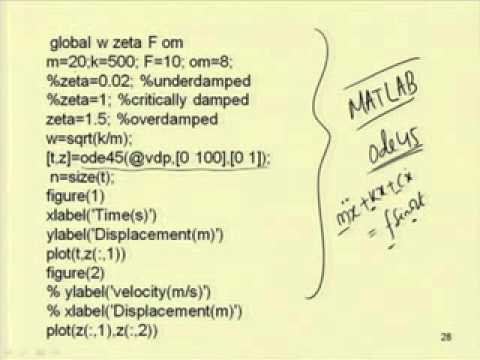
Or one can develop a code, using this MATLAB to find the response. So, in MATLAB a function
ode 4 5, one may use to solve these equations. So, this equation may be one can solve a linear
equation or non-linear equations; so one can write a simple code in MATLAB to find this.
So, here let us use this equation or use this MATLAB function to solve this linear equation
first. So, let us solve this equation m x double dot plus k x plus c x dot equal to
f sin or cos omega t f sin omega t. So, in this case for a given value of m k c and f
and omega, one can find x. So, first one has to reduce this equation, this second order
equation to a set of first order equation; so after reducing this equation to a set of
first order equation, one can find it is solution. So, to reduce this thing into a set of first
order equation, so one can write this equation in this form.
So, one can write this equation ok. So, let me write this equation, so the equation is
m x double dot plus k x plus c x dot equal to f sin omega t. So, one can write this x,
let one put this x dot equal to z 2 and x equal to z 1. So, if one substitute x equal
to z 1 and x dot equal to z 2, then this equation can be written in this form. So, x dot equal
to z 2 or one can write this x double dot equal to f sin omega t minus k x minus e x
dot, so this thing can be written this x double dot as x dot is written z 2, so this x double
dot equal to d z 2 by d t. So, this is d z 2 by d t, so this will be equal to so d z
2 by d t will be equal to f sin omega t minus k. So, for x 1 put this equal to z 1 minus
c, for x dot 1, put it z 2 or this equation this equation also can be written in the form:
x double dot plus omega n square x plus 2 zeta omega n x equal to f by m sin omega t,
so this f by m can be written in this form.
So, x double dot plus omega n square x plus 2 zeta omega n x equal to f sin omega t, so
substituting this x equal to z 1, and x dot equal to z 2.So, one can get two differential;
first order differential equation: the first differential equation is this one, that means
d z 1 by so, first differential equation equal to d z 1 by d t equal to z 2, and second equation
becomes, d z 2 by d t, so this becomes f sin omega t minus omega n square x minus 2 zeta
omega n 2 zeta omega n x dot. So, by putting these two equation in a function, so here
in MATLAB; this function written is written as, v d p. So, function d z equal to v d p
t z and using this global value this or this w represent this omega n, and this zeta f,
f is the amplitude of the expectation, and omega o m is the frequency of this excitation.
So, by putting this as global variable, so one can write d z equal to 0, so initially
it as, we have two equations. So, we can put it 0’s to 1, so d z 1 equal to z 2, this
is the first equation. And, the second equation is written d z 2 by d t; as d z 2 equal to
f sin omega t minus 2 zeta omega z 2 minus omega square z 1. So, using this function
one can find, one can use this function in this ode 45; this is the command for finding
this thing. So, d z equal to omega o d e 45 v d p, so by taking this initial condition,
so one can take the time step and initial condition and find the response of the system,
so taking it 0 to 100 time step.
And, 0 to 1 as the initial condition, so one can find the response, so n equal to by putting
this n equal to size t. So, here so 3 cases have been solved; one first case by taking
m equal to 20, k equal to 500, f equal to 10, and omega equal to 8. So, the response
have been found for the under dumped case by taking zeta equal to 0.02 ,critically damped
case zeta equal to 1, and zeta equal to 1.5 for the over damped case. So, the response
curves have been plotted both in phase portrait and time response.
So, let us see this thing. So, for a under damped case so for a under damped case: one
can see the initial part, which represent the transient part of the response, so it
is varying with the initial condition, and it decreases, and finally it approaches a
steady state response. So, this is the state response raised after several time steps.
So, one can find the steady state response by using this method also, this is the transient
part, this is the steady state part and this shows the time response of the system.
So, one can find the time response for the critical critically damped case. So, this
is represent the critically damped case; so here the displacement in meter, and time in
second. Similarly, one can find the response for the over damped case.
And, if one plot the phase portrait; so this phase portrait is plotted along with the transient
part. That is why, it shows both transient and the steady state response part. This curve
shows, the steady state part and starting for a initial condition. So, this shows the
both transient and steady state part for this damped condition.
And, for the critically damped condition, so this response, this phase portrait represent
the phase portrait for the critically damped case. And this represent for the under damped
case.
So let us see, three more examples. So, in this case instead of taking a single forcing
function, if one take two forcing function, so this is a 2 frequency excitation case.
So, in this case one can note that, this x double dot plus 4 x plus 0. 2 x 0. 2 x dot;
here this 4 is the omega n square, so omega n equal to 2. The nature frequency of the
system equal to 2. And in this case, it is subjected to a excitation with a frequency
2 and 4 and with amplitude 5. In the second example: So, it is subjected to a frequency
of 3 and 3 root 2, and in the third example: it is subjected to a frequency of 1 and 0.99.
So, in the first case one except to have two periodic response; one corresponding to this
2 t, and other one corresponding to the 4 t, corresponding to omega equal to 2, and
other correspond to omega equal to 4. But, in the second case as the ratios are irrational
number; so that means 3 root 2 by 3 equal to root 2.
So, one can get a quasi periodic response in the solution. In the third case, the response
will be a periodic or one can get a beating type of response, as the frequencies are very
near to each other, so this is 1 and this is 0.99. So one has a beating frequency of
0.01.So, by using this Runge-Kutta method, the response have been plotted, so in the
three cases it has been plotted.
So, this is the phase portrait and time response. So, quasi periodic response and so, this is
the phase portrait for the quasi periodic response; and this is the response for the
beating type of beating type beating phenomena. This shows the constructive and destructive
inference type of things, and when one has frequency nearly equal to so, the as the beating
frequency is 0.1; this shows the response, and one find the amplitude; maximum amplitude
and minimum amplitude. In this case, so by using this method this Runge-Kutta method,
one can find the time response, phase portrait of the system. So, in addition to finding
this equation of the linear system, one can use the same equation for the non-linear case
also.
Let us take, the doffing equation. So, in case of the doffing equation; so x double
dot plus, let us take a equation in this form: x double dot plus omega 0 square x plus 2
zeta omega n x dot plus alpha x cube, let it is equal to f sin omega t, so in this case,
so one can write those two function; that is d z 1 equal to z 2, and the second equation
d z 2.
One can write this in this form, so it will be f sin omega t minus omega 0 square z 1
minus 2 zeta omega n z 2 minus alpha z 1 cubed, but it may be noted, that in this case as
one can have multiple solutions. Unlike in case of the linear system, what we have seen
before, so it depends on the initial condition. What we are supplying to the system? So, while
solving so depending on the different initial conditions, so one can have different phase
portraits and different time response of the system.
So later, when we study about different resonance conditions, and then we will know that. This
equation will have many different types of solution, depending on the resonance conditions,
and for that matter, for a particular value of forcing frequency omega, for a particular
value of forcing frequency omega as it have several solutions. So, one can plot or one
can plot the phase portrait, in which taking different initial conditions. One can have
the equilibrium positions.
So, one can find the equilibrium position, so by using this Runge-Kutta method. So, one
can find the steady state solution, and as it has several solutions; so depending on
the initial condition; it will go to a particular solution. So, this plot, which shows the variation
of the trajectories depending on the initial conditions are known as basin of attraction
basin of attraction.
So, by plotting this basin of attraction, so one can find so one can find the trajectories
starting form a particular point and ending at the equilibrium position. So, this basin
of attraction there are several methods to plot, this basin of attraction. So, which
we will study in later module but, one may note that, the methods may be a point to point
mapping method, point to point mapping or cell to cell mapping method. So, one can use
either a point to point mapping method or cell to cell mapping method, to plot this
basin of attraction for a non-linear system. To find all the equilibrium positions. So
later, we will see how to solve this equation by using this Runge-Kutta method and qualitatively
qualitatively.
Already, we have seen one example of the Duffing equation, to plot the phase portrait and to
study the phase portrait also graphically. There are several methods available to study
this phase portrait. So, one such method is the method of isoclineso. In case of, method
of isoclines, so one can let us see the method of isoclines.
And so, there are several methods. So, one method is method of isoclines, second method
is delta method. Then, we can have the modified delta method and we can have the double delta
method. So, today class we will see about this isocline method. And, then we will study
the straight forward expansion method. So, in case of method of isoclines; iso means
similar or equal, so isocline method one has to plot lines with equal slopes, and draw
the phase portrait. So let us consider, this equation u double dot plus omega square u
equal to f u u dot and t.
So, in this case by taking v equal to d u by d t. So, one can write this u double dot
equal to d by d t of u dot, so this is equal to d v by d t equal to, one can write this
is equal to d v by d u into d u by d t, and as we are taking this d u by d t equal to
v. So, one can write this u double dot equal to v into d v by d u, so by taking this equation
or substituting this equation in the first equation, one can write v d u by d t equal
to f u u dot t minus omega square u or this d v by d u equal to f u u dot t minus omega
square u by v as d v by d u, represent the slope of the trajectory in the phase portrait.
So, one can plot this phase portrait in u v plane, and one can find this phase portrait.
So, for example let us take the equation, u simple linear equation: u double
…
will continue, the solution procedure of the non-linear equations; and in the previous
class, we have reviewed or we know about, what is a solution or equilibrium points,
types of equilibrium points, representation of the solution, and how solution of a linear
and non-linear systems differ? And how to determine the solution? So, in the last class
I told you, to determine this solution, so we can apply or we can go for a qualitative
analysis or we can have this quantitative analysis.
So, in case of the qualitative analysis, we have seen how to plot the phase portrait to
find the response of the system? And also to find the equilibrium points, let us take
few examples: few more examples and let us see, how to how these equilibrium points are
determined?
For example, so let us take this example: Let, we have a equation x double dot plus
x minus 0.1 x cube equal to 0. So, as told before in case of the equilibrium position,
or in case of the equilibrium solution, so if it is steady state solution, then it will
not be a function of time. So, this x double dot or any function of any variation of x,
with time should be neglected, so in this case, we can neglect this x double dot equal
to put x double dot equal to 0.
And the remaining thing, we can write as x minus 0.1 x cube equal to 0; and this will
give rise to x into 1 minus 0.1 x square equal to 0 or so, in this case we can have this
x either x equal to 0 or, this 1 minus 0.1 x square equal to 0, which will give rise
to x square equal to 10 or x equal to plus minus 3.1627. So, in this case, we have 3
values of this x so, these 3 are the equilibrium position for this equation.
So in this equation, x equal to 0 refers to the trivial solution, and x equal to plus
minus this 3.1627 are the non trivial solution of the system. So, one can use this qualitative
analysis procedure, to find the phase portrait of this equation, and one can check, whether
these points correspond to this center saddle point? and one can find the separate ricks
also in this case? So, let us take another example: So in this case, let us take this
equation. In this form, x double dot minus x plus 0.1 x cube equal to 0. So, in the previous
case, the this is similar to, this doffing equation with a subtending type of spring
with cubic nonlinearity. This is we have this minus 0.1 x cube.
And in this case, we have taken a equation, we have this linear stiffness part is written
as negative. So, in this case for this steady state solution, this x double dot will be
equal to 0, and this equation can be written as so x minus 0.1 x cube equal to 0. So, we
can have the solution x or x into 1 minus, so x into 1 minus 0.1 x square equal to 0
or, we can have x equal to 0 and x equal to plus minus 3.1627. So in this case also, we
have same solution; that is x equal to 0 is a solution and x equal to plus minus 3.1627
another two solutions; so these are the equilibrium points of this equation.
So, let us take another example; so in this case; so let us take the example; example
3: So, in this case u double dot plus omega 0 square u equal to epsilon into u dot minus,
let me take this u dot u cube. So, in this case for steady state, one can put this u
dot and u double equal to 0. So by putting, u dot and u double dot equal to 0. So, one
can obtain the equilibrium solution as omega 0 square u equal to 0 or u equal to 0. So,
this u equal to 0 represents the equilibrium solution in this case.
So, one can obtain; so this is the 100 pole equation, and the previous two equations are
doffing equations. And, one can obtain the response of the system by using qualitative
analysis or quantitative analysis. And today class, we will see, how you can use a straight
forward expansion method for find the solution of the system? Also, one can go for this numerical
analysis method, or numerically, one can solve these equations to obtain the solution of
the system. And, let us take another example: In which, one has to plot this potential or
one has to do the qualitative analysis for a simple pendulum.
So, in case of the simple pendulum, the equation can be given. So, in case of a simple pendulum,
the equation motion of this, so this has a mass m, and so the system has a mass m and
length is l. So, the equation of motion can be written as theta. So if it is moving with
theta, this equation is theta double dot plus omega square sin theta equal to 0. So, where
omega square equal to g by l, so g is acceleration due to gravity, and l is the length of the
simple pendulum.
So, in this case, so if one do this qualitative analysis, so here one can find this f theta
equal to, that is the potential function equal to integration of this f u d u. So that means,
integration of this omega square sin theta d theta, so that thing can be written in this
form. So, omega square cos theta, so the equation can be written by integrating this equation.
Already you we know, that it can be written in this form. So, ½ theta dot square plus
f theta will be equal to h or one can write this equation, or one can write this theta
dot equal to root over 2 into h minus omega square cos phi. Here, one may note that, unlike
in case of simple degree of freedom system, when we are taking sin theta equal to theta,
here one can takes this instead of taking sin theta equal to theta, one can expand or
one can take it directly.
And, one can find this expression for theta dot equal to 2 into h minus omega square cos
theta. So, for different value of h, so one can plot this flow, that is theta dot. And,
one can find the equilibrium position. For example: In this case, the equilibrium position,
one can have two equilibrium position one, so by putting this theta double dot equal
to 0. The equilibrium position corresponds to sin theta equal to 0.So, sin theta, so
these correspond to sin theta equal to 0. So, in this case sin theta equal to 0, at
theta equal to 0 and 180 degree. And so, one can have two positions; so this is one equilibrium
position and the other equilibrium position will be this one. So, one can have two equilibrium
position, one correspond to theta equal to 0 and other correspond to theta equal to phi.
So, it may be so when, we will study the stability analysis or when we will carry out the stability
analysis of the system, we can see that this equilibrium position is a stable equilibrium
position, while the other equilibrium position is an unstable equilibrium position. So, this
equilibrium position represent in the absence of this damping. So, this will represent a
center and the motion will be periodic. So, one can have a periodic motion but, this equilibrium
position will be an unstable saddle point. So, one can plot this theta dot versus this
theta to qualitative analyze, the throw or trajectory of this system.
And, one can do this numeric. Last class several methods has been pointed out, which can used
for solving this non-linear equation motion. So, these methods include the straight forward
expansion method, harmonic balance method, lindstedt Poincare method, method of averaging,
method of multiple scales, intrinsic harmonic balance method, generalizing harmonic balance
method, multiple time scale harmonic method and modified lindstedt-Poincare method. And
before, studying this straight forward expansion, let us take or let us study about the numerical
methods are by using the numerical method. We can find the solution of these equations.
So, in case of the numerical method, let us take this Runge-Kutta method, for Runge-Kutta
4th order method for finding the solution.
So in this case, in case of the Runge-Kutta method, so one can solve this initial value
problem d y by d x. In this form, d y by d x equal to f x y, where y a equal to y 0,
and this a will be within a and b. So, this d y by d x while solving this equation, d
y by d x equal to f x y. So, it has four steps; so one can find the k plus 1 eth solution
as a function of k eth solution as follows; so y k plus 1 will be equal to y k plus k
1 plus 2 k 2 plus 2 k 3 plus k 4 by 6, where k equal to h into function of x k and y k.
So, in this case this k 2 can be written as h into f x k plus h by 2 y k plus k 1 by 2.
So, this function evaluated at, x k plus h by 2 and y k plus k 1 by 2, will be used to
find this k 2 constant k 2, similarly constant k 3 can be found by putting this or evaluating
this function at x k plus h 1 by 2 and y k plus k by 2 k 2 by 2; so this is k 2 and this
is k 1 and this k 4 also can be obtained. So, by using this k 1, k 2, k 3, k 4 in this
equation, so one can evaluate this y k plus 1 as a function of y k. And, one can find
the solution of any governing equation of motion, any differential equation motion.
Or one can develop a code, using this MATLAB to find the response. So, in MATLAB a function
ode 4 5, one may use to solve these equations. So, this equation may be one can solve a linear
equation or non-linear equations; so one can write a simple code in MATLAB to find this.
So, here let us use this equation or use this MATLAB function to solve this linear equation
first. So, let us solve this equation m x double dot plus k x plus c x dot equal to
f sin or cos omega t f sin omega t. So, in this case for a given value of m k c and f
and omega, one can find x. So, first one has to reduce this equation, this second order
equation to a set of first order equation; so after reducing this equation to a set of
first order equation, one can find it is solution. So, to reduce this thing into a set of first
order equation, so one can write this equation in this form.
So, one can write this equation ok. So, let me write this equation, so the equation is
m x double dot plus k x plus c x dot equal to f sin omega t. So, one can write this x,
let one put this x dot equal to z 2 and x equal to z 1. So, if one substitute x equal
to z 1 and x dot equal to z 2, then this equation can be written in this form. So, x dot equal
to z 2 or one can write this x double dot equal to f sin omega t minus k x minus e x
dot, so this thing can be written this x double dot as x dot is written z 2, so this x double
dot equal to d z 2 by d t. So, this is d z 2 by d t, so this will be equal to so d z
2 by d t will be equal to f sin omega t minus k. So, for x 1 put this equal to z 1 minus
c, for x dot 1, put it z 2 or this equation this equation also can be written in the form:
x double dot plus omega n square x plus 2 zeta omega n x equal to f by m sin omega t,
so this f by m can be written in this form.
So, x double dot plus omega n square x plus 2 zeta omega n x equal to f sin omega t, so
substituting this x equal to z 1, and x dot equal to z 2.So, one can get two differential;
first order differential equation: the first differential equation is this one, that means
d z 1 by so, first differential equation equal to d z 1 by d t equal to z 2, and second equation
becomes, d z 2 by d t, so this becomes f sin omega t minus omega n square x minus 2 zeta
omega n 2 zeta omega n x dot. So, by putting these two equation in a function, so here
in MATLAB; this function written is written as, v d p. So, function d z equal to v d p
t z and using this global value this or this w represent this omega n, and this zeta f,
f is the amplitude of the expectation, and omega o m is the frequency of this excitation.
So, by putting this as global variable, so one can write d z equal to 0, so initially
it as, we have two equations. So, we can put it 0’s to 1, so d z 1 equal to z 2, this
is the first equation. And, the second equation is written d z 2 by d t; as d z 2 equal to
f sin omega t minus 2 zeta omega z 2 minus omega square z 1. So, using this function
one can find, one can use this function in this ode 45; this is the command for finding
this thing. So, d z equal to omega o d e 45 v d p, so by taking this initial condition,
so one can take the time step and initial condition and find the response of the system,
so taking it 0 to 100 time step.
And, 0 to 1 as the initial condition, so one can find the response, so n equal to by putting
this n equal to size t. So, here so 3 cases have been solved; one first case by taking
m equal to 20, k equal to 500, f equal to 10, and omega equal to 8. So, the response
have been found for the under dumped case by taking zeta equal to 0.02 ,critically damped
case zeta equal to 1, and zeta equal to 1.5 for the over damped case. So, the response
curves have been plotted both in phase portrait and time response.
So, let us see this thing. So, for a under damped case so for a under damped case: one
can see the initial part, which represent the transient part of the response, so it
is varying with the initial condition, and it decreases, and finally it approaches a
steady state response. So, this is the state response raised after several time steps.
So, one can find the steady state response by using this method also, this is the transient
part, this is the steady state part and this shows the time response of the system.
So, one can find the time response for the critical critically damped case. So, this
is represent the critically damped case; so here the displacement in meter, and time in
second. Similarly, one can find the response for the over damped case.
And, if one plot the phase portrait; so this phase portrait is plotted along with the transient
part. That is why, it shows both transient and the steady state response part. This curve
shows, the steady state part and starting for a initial condition. So, this shows the
both transient and steady state part for this damped condition.
And, for the critically damped condition, so this response, this phase portrait represent
the phase portrait for the critically damped case. And this represent for the under damped
case.
So let us see, three more examples. So, in this case instead of taking a single forcing
function, if one take two forcing function, so this is a 2 frequency excitation case.
So, in this case one can note that, this x double dot plus 4 x plus 0. 2 x 0. 2 x dot;
here this 4 is the omega n square, so omega n equal to 2. The nature frequency of the
system equal to 2. And in this case, it is subjected to a excitation with a frequency
2 and 4 and with amplitude 5. In the second example: So, it is subjected to a frequency
of 3 and 3 root 2, and in the third example: it is subjected to a frequency of 1 and 0.99.
So, in the first case one except to have two periodic response; one corresponding to this
2 t, and other one corresponding to the 4 t, corresponding to omega equal to 2, and
other correspond to omega equal to 4. But, in the second case as the ratios are irrational
number; so that means 3 root 2 by 3 equal to root 2.
So, one can get a quasi periodic response in the solution. In the third case, the response
will be a periodic or one can get a beating type of response, as the frequencies are very
near to each other, so this is 1 and this is 0.99. So one has a beating frequency of
0.01.So, by using this Runge-Kutta method, the response have been plotted, so in the
three cases it has been plotted.
So, this is the phase portrait and time response. So, quasi periodic response and so, this is
the phase portrait for the quasi periodic response; and this is the response for the
beating type of beating type beating phenomena. This shows the constructive and destructive
inference type of things, and when one has frequency nearly equal to so, the as the beating
frequency is 0.1; this shows the response, and one find the amplitude; maximum amplitude
and minimum amplitude. In this case, so by using this method this Runge-Kutta method,
one can find the time response, phase portrait of the system. So, in addition to finding
this equation of the linear system, one can use the same equation for the non-linear case
also.
Let us take, the doffing equation. So, in case of the doffing equation; so x double
dot plus, let us take a equation in this form: x double dot plus omega 0 square x plus 2
zeta omega n x dot plus alpha x cube, let it is equal to f sin omega t, so in this case,
so one can write those two function; that is d z 1 equal to z 2, and the second equation
d z 2.
One can write this in this form, so it will be f sin omega t minus omega 0 square z 1
minus 2 zeta omega n z 2 minus alpha z 1 cubed, but it may be noted, that in this case as
one can have multiple solutions. Unlike in case of the linear system, what we have seen
before, so it depends on the initial condition. What we are supplying to the system? So, while
solving so depending on the different initial conditions, so one can have different phase
portraits and different time response of the system.
So later, when we study about different resonance conditions, and then we will know that. This
equation will have many different types of solution, depending on the resonance conditions,
and for that matter, for a particular value of forcing frequency omega, for a particular
value of forcing frequency omega as it have several solutions. So, one can plot or one
can plot the phase portrait, in which taking different initial conditions. One can have
the equilibrium positions.
So, one can find the equilibrium position, so by using this Runge-Kutta method. So, one
can find the steady state solution, and as it has several solutions; so depending on
the initial condition; it will go to a particular solution. So, this plot, which shows the variation
of the trajectories depending on the initial conditions are known as basin of attraction
basin of attraction.
So, by plotting this basin of attraction, so one can find so one can find the trajectories
starting form a particular point and ending at the equilibrium position. So, this basin
of attraction there are several methods to plot, this basin of attraction. So, which
we will study in later module but, one may note that, the methods may be a point to point
mapping method, point to point mapping or cell to cell mapping method. So, one can use
either a point to point mapping method or cell to cell mapping method, to plot this
basin of attraction for a non-linear system. To find all the equilibrium positions. So
later, we will see how to solve this equation by using this Runge-Kutta method and qualitatively
qualitatively.
Already, we have seen one example of the Duffing equation, to plot the phase portrait and to
study the phase portrait also graphically. There are several methods available to study
this phase portrait. So, one such method is the method of isoclineso. In case of, method
of isoclines, so one can let us see the method of isoclines.
And so, there are several methods. So, one method is method of isoclines, second method
is delta method. Then, we can have the modified delta method and we can have the double delta
method. So, today class we will see about this isocline method. And, then we will study
the straight forward expansion method. So, in case of method of isoclines; iso means
similar or equal, so isocline method one has to plot lines with equal slopes, and draw
the phase portrait. So let us consider, this equation u double dot plus omega square u
equal to f u u dot and t.
So, in this case by taking v equal to d u by d t. So, one can write this u double dot
equal to d by d t of u dot, so this is equal to d v by d t equal to, one can write this
is equal to d v by d u into d u by d t, and as we are taking this d u by d t equal to
v. So, one can write this u double dot equal to v into d v by d u, so by taking this equation
or substituting this equation in the first equation, one can write v d u by d t equal
to f u u dot t minus omega square u or this d v by d u equal to f u u dot t minus omega
square u by v as d v by d u, represent the slope of the trajectory in the phase portrait.
So, one can plot this phase portrait in u v plane, and one can find this phase portrait.
So, for example let us take the equation, u simple linear equation: u double
…