en English
Untitled English subtitles
Report a problem
Advertisement
English transcript
Hello everybody. Let us continue our lecture series in this course, optimal control guidance
and estimation. We are here at lecture number 5, where we are talking about some sort of
overview of static optimization and this is part 2 of the lecture actually. So, very quickly,
I mean we can just see what all we discussed in the last lecture before coming to this
one actually.
So, we talked about some sort of unconstrained optimization followed by some some constrained
optimization with equality constraints and then, saw some numerical examples on the way.
So, these are all what we discussed, I mean taking, getting motivated from a simple, I
mean simple curve sort of thing and analyzing those points.
Then, finally analyzing whether the derivative is 0 or not. Then, it turns out after rigorous
analysis through Tailor series that the first derivative needs to be 0. Then, we continued
further with second derivative, third derivative and so on.
You just tends out that for for necessary conditions, all odd derivatives needs to be
0 and for sufficiency condition can be arrived at with even powers and all that, with the
sine sensitivity all that. So, all these things we have discussed in the last lecture anyway.
We saw some examples on the way and then, followed to this vector case where the decision
variables are actually x 1 to x n number of variables.
In that case, you will have to define some radiant vector and then, asymmetric things
like that and again, they are using the same idea of Ruler series.
Then, we arrived at a conclusion that if the, so the necessary condition the radiant vector
needs to be 0 and sufficiency condition can be arrived by looking at the positive definiteness
or negative definiteness of this isometric actually and again, followed with some examples
and all that it will appear.
Then, we moved on to some constrained optimization with equality constraint and then, we told
that this particular problem, the minimize J of x subject to the f of x equal to 0 is
equivalent to minimizing this J bar of x and lambda, where both x and lambda are considered
as p variable.
We constrained this function and then, use the analysis tools that you know for unconstrained
optimization for J bar. With that in and then, connect with these 2 necessary condition again
and went through the example problems.
Finally, I mean we went some sufficiency condition as well and told that you have to construct
this kind of a matrix. Then, see the determinant and interpret that is the function of only
sigma’s and analyze the the sine sensitivity of all these sigma’s actually.
If all of them appear to be positive, it is the least minimum condition and all of them
appear to be negative, then it is a maximum condition actually.
Again, we demonstrated that using some some examples and all that actually, all right.
Then, we had a good example at the end, where took out this x 1 minus x 2 square and then,
constraint values of a non-linear equation and it will ended up with some multiple cases.
Depending on each other cases, we had analyzed this particular equation. Then, using that
case one, what you got here? We got some some results that sigma equals to minus 3 and hence
that leads to maximum and all that actually.
So, for considering and analyzing all these things for all the roots, we had a conclusion
that these two will lead to maximum and these two lead to minimum. If we really want to
have global maximum and global minimum ideas, then at this point, you have to evaluate the
J, both both the points and whichever J appears to be maximum is a global maximum.
Then, these two you can evaluate the function J and whichever appears to minimum, appears
to be a global minimum. So, that was the idea there actually. Then, we write some references
and then, I suggested to look at some books and all that. So, that was our last lecture.
Now, coming to this particular lecture, we will talk about constraint optimization with
mainly inequality constraints and also before moving on, we will also have a glimpse of,
a small glimpse of numerical optimization techniques. Especially, this this stiffest
designed method and this Newton’s like that usually we will see something. Those are the
things that break one of any optimization techniques including dynamic optimization.
That means optimal control areas. So, we have to, we will just have a glimpse of it.
Well, again this is not a course on static optimization. So, we will not deal over there.
We will not take a lot of time to kind of analyze various techniques and all that. At
least good to have some idea of what is numerical optimization actually. Then, we will follow
up with some numerical examples before winding up this lecture. All right. So, constrained
optimization with inequality constraints, that is what we want to see first analytically
and then, we will see some numerical things and all towards end of this lecture actually.
So, one very quick way of an inequality constraint approach or other I will call that as a naïve
approach, say something like this. We will visualize a problem where if this variable,
decision variable, all of them are constraint like this let say. So, all of x i or x 1,
x 2, x 3 all that are the constraint between their corresponding minimum and maximum values.
Then, how do you handle that problem?
One easy idea or other make approach that turns out be, like ok you will construct some,
I mean you just replace this x i, where something like this, where x i, I mean now you interpret
alpha i as a free variable. That mean, if one no matter whatever is the value of alpha
is, note that sine square alpha is always bounded between 0 and 1. So, it happens to
be 0, then x i turn out to be minimum and if happens to be 1, then it turns out to be,
these 2 will be cancelled out and it will turn to be maximum value.
So, no matter whatever the value is of alpha i, your x i will be bounded between these
2 things actually. So, that is the one idea, but also note that we have actually introduced
a nominal transformation here and this x i and alpha i are not really linearly related.
You have this human less problem of like so many local variables and so many values of
alpha i, which will give it to that actually because sine square alpha i is not here. I
mean, it is not uniquely valued and all I mean, it is not a unique function sort of
things like that. So, we will end up with a huge amount of problem
here because most of the time, if you just do it and carry of numerical optimization
which typically we have to do at the end of the day, then it is not a very good way of
doing that. Also, a simple problem can get translated into a very complex problem through
this early on transformation if you want to do it through analytical tools actually.
So, this is even though, it is a very lucrative approach and you can probably try out at the
first go, It is not really universal solution that we are looking for actually. So, this
approach in general does not work. If you can try it out, we do I mean in a given problem
you can try it out. If it works out, nothing like that, but in general, it does not work
out very well actually. So, we are in a process of pointing out for better approaches usually.
So, let us see that, I mean first the problem definition. What you really want here is minimize
or maximize this J of x. Again, the cost function or objective function is always a scalar,
but the decision number of free variables can be, I mean n dimension. That means, we
have n number of free variables to choose from in a difference in combinations and all
that, but this particular objective function is now subject to this, this constraint g
1 to g m less than equal to 0. Now, remember this also inverse to this inequality
constraint because we are considering less than equal to 0 here. If it equal to 0, then
it all satisfy that. So, that means, what we discussed in the previous lecture in inequality
constraints is a kind of embedded over here actually ok, but we have talking in more general
thing. That mean, first first couple of equations inequality constraints. We are assured that
constraints are not really equality; they are inequality constraints in a way actually
ok. So, how do you handle that in general? Now,
consider I mean this particular problem that this is or less than equal to 0. So, the one
approach is to introduce something called slack variables, ok mu 1 to mu m, all all
are considered as slack variables to convert the inequality constraints to equality constraints
because they are less than 0. So, I can always add a number there and just to make sure that
we have positive quantities, I will added something like mu 1 square, mu 2 square up
to mu m square actually ok. So, if I do that, it turns out that it is
is nothing, but inequality constraints problem actually. Then, the idea is to follow up the
routine procedure for the equality constraints because we know how to handle the equality
constraints analytically. We we can carry further and then, proceed further actually.
However, not that is even though, it is less than equal to 0, not that we really do not
know how far it is away from 0. So, these values of mu 1 to mu m is typically not known.
I mean that even though symbolically you can write it that way. Using it for inferring
something is not really very nice because you will not be aware of any idea of this
number actually.
So, we want some conditions which are independent of at the final relations actually. So, let
us see whether you can really do that or not actually. Anyway, so this is a problem of
maximize or minimize J of x now subject to this constraint, which is equality constraint
ok. So, this is what you are doing. So, now, if you look at this one and then, equality
constraint, we know how to handle that. So, first to construct J bar and now J bar is
a function of x and lambda, but also these mu is free variable, slack variable actually.
So, this actually is a function of all these quantities, x lambda and mu ok.
So, this is constructed that way. So, as far a necessary condition is concerned, I mean
concerned, we have to take take partial derivatives with respect to all these variables, x lambda
and mu. X is n dimensional quantity whereas, lambda and mu you remember lambda and mu are
given by dimension of the constraint equations and that is typically m basically. So, we
will consider these n derivates here coming from x i, partial derivatives that has to
be equal to 0 and then, finally followed by this del J bar by del lambda J which is like
free variable of lambda considering that free variable lambda here here we talked about
that actually ok. So, this is the second equation and then,
we have a free variable with mu and that mu turns out to be like this del J bar by del
mu, that has to be equal to 0 in case. So, these conditions what you are getting n, n
equations, m equations and m equations, that is n plus 2 m equations have to be solved
to get that basically and we get the idea there actually. I mean we will get the solutions
what we want to achieve. We have to utilize the equations now. How do you do that? So,
let us analyze little more. So, this equation let us start with for second one.
So, this turns out to be 0. Hence, g j of x, I can write it to a negative of u j square
actually. Now, if I multiply those sides with lambda j, I can write it that way, but remember
that this particular equation comes under now lambda j mu j equal to 0 now. So, what
it tells us this this quantity 0. Hence, lambda j into g j has to be 0 ok. Just if if I take
this equation and get g j x, the negative mu square mu j square, multiply both sides
lambda j and then, use a third equation. What I am having here? So, once I get that, then
it tends out that g j lambda j is nothing, but is 0.
So, this leads to the conclusion that either lambda j 0 or g j 0. Now, if lambda j is 0;
that means, the constraint is kind of inequality I mean strictly inequality constraint, which
means the constraint is not acting. That means, it is actually a kind of and you can visualize
as if the constraint is not there actually, lambda j 0 you do not because that is coming
through this constraint equation but because you have a constraint equation, you have that
and then, it is coming through that. So, if lambda j is 0 for a particular thing, you
can visualize very well as if the constraint is not there actually, but that is a mathematical
interpretation actually. So, if otherwise g j is equal to 0; that means,
it is active constraint. Now, if we go back to here, the g j becomes equal to 0, it becomes
an active constraint. So, if the problem is, I mean either the constraint g j is not there
and it is as good as not there or it takes as a kind of active constraint actually. So,
that is the conclusion here which makes a lot of sense actually. If I mean, if g j is
strictly less than 0, then we can very well forget it actually and then, try to optimize
only the actually or anyway, this is the conclusion here. So, lambda j g j equal to 0, that leads
to the conclusion that either lambda j 0 or g j 0. That means, putting in English words
if a constraint is strictly an inequality constraint, then the problem can be solved
without considering it. Otherwise, the problem can be solved by considering it as a strictly
equality constraint. So, that is the conclusion here, but it also gives us a procedure to
solve now. Let us say, how to do that? Now, notice that
this equation has nothing to do with the mu actually. This this equation is simplified
to deal with lambda’s and g’s actually. So, really we do not need to know the value
of mu now, all right. So, now to consider this this analysis further, let us talk about
a single, I mean typical case, the typical maximization problem. I mean remember it is
not minimization problem we are considering, we are considering the maximization problem
and g j is active. That means g j is equal to 0 actually.
So, how do you conclude in that particular situation, what is happening there? Now, let
us assume that x is a point where maximization or maximum occurs, maximum of the cost value
occur and delta x i is a small change in x i direction that causes g j to be strictly
negative. That means, the moment that I will go a little bit in that particular direction,
my g j becomes inactive actually. In that situation only, we have got the optimization
optimal point basically that happens, all right.
So, at that point the maximum occurs and it may in a particular direction of delta x i
g j tends out to be strictly negative. That means, from active constraint, it becomes
inactive constraint actually. So, that is the point where maximization occurs. Now,
how do you handle? I mean how do or what do you infer from there actually?
So, if we go back to d j, it tends out to be like that, del j by del x y into delta
x y actually. Remember, it is g j is active actually. So, this is d j is nothing, but
del j by del x i into delta x i. This is less than 0. Since, g j maximum point actually
in that sense and then, because this particular direction, any direction I go from that particular
thing, this has to decrease. That is a pre-optimization problem, but in a constraint optimization
sense, it may not happen. We are not allowed to go to one side, but whatever direction
we are allowed to go, if we go to any direction, any direction within that allowable zone,
then we are suppose to decrease, I mean the cost function also decreases actually.
Then, this also becomes true because d j and d of g j are nothing, but something like this.
In that particular direction turns out to be less than 0 from this inference actually.
Thus, g j tends to be less than 0 actually here. So, from that it it turns out that this
this condition is also true here. So, now, what you infer from this actually? So, if
if these two conditions are true now, let us consider delta x i is a positive quantity.
It can very well be negative quantity which is to be discussed here next.
If it is positive quantity, then what happens? We have to satisfy these conditions anyway.
So, that means, del j by del x i and del g j by del x i has to be negative quantities.
Then only, this this equation will be holding true. Now, if this happens to be a negative
quantity, again opposite is true. Now, these, both of them have to be positive quantity
now. I mean the noticed, I mean the thing to note here is, both of them has to be either
negative or both of them has to be either positive. That is the conclusion for a maximization
problem, remember. Now, if it is a minimization problem, this sign will alter. This will become
positive here and then, their inferences has to both held to be like kind of an opposite
sign each other and all that actually. Now, let us not worry about that. We are considering
a maximization problem and this is what happens. Both the things will take the same sign basically
now. What do you conclude from there? Now, you will go back. So, for we have been dealing
with these 2 equations. We never thought about that equation, I mean using that equation
so far.
So, we will go back to that and see what you can get from there. Now, you remember this
this quantity and this quantity has to be of same sign basically. That is what we have
just discussed it actually. Now, going back to this, this is what we are getting here.
That means, del j by del x i equal to that one. I will take that in other side of the
story and because lambda j, I mean all that I can inform you here lambda j is not a function
of x. So, I can take it out from there and it turns out that these gives us another constraint
equation, that this partial derivate and this partial derivative are related to each other
through that, but these two quantities are always having same sign and with a negative
quantity here. That means lambda j has to be a negative. Remember this analysis told
us that these two will always have the same sign, no matter whether the delta x i is positive
or negative. So, if we have the same sign and this is a constraint equation with a negative
sign, then lambda j has to be negative of each other, then only it will satisfy all
that.
So, this is what it tells us. It tells us what if it is a maximization problem, right.
I mean that is right, if that is a maximization problem, then these two, I mean this lambda
j has to be a negative basically ultimately. So, this this kind of analysis you can do
case by case and generalize things like that.
So, as summary sort of things, this this kind of analysis is called something like, earlier
it was known as Kuhn Tucker condition and some books still follow that, but more popularly,
now it is known as Karush Kuhn Tucker condition. The Karush Karush happens to be the independent
results actually and then, Kuhn tucker divided these conditions. It become popular and later
they realize that I think Kuhn-Tucker themselves or somebody else in the process of analysis,
they realized that Karush is actually developed this condition as a part of the master pieces
and then, the story goes on like that actually. So, then they want to attach his name further
and things like that and they prolonged here is Karush published his results. It became
part of his thesis only. So, somewhat it was discovered, otherwise it would have been simply
Kuhn Tucker condition all the time actually. So, I mean that also uses the clue that whenever
you get something, try to publish. Please do not keep it yourself whether that actually
anyway. So, this this is the condition here which is popularly known as KKT conditions
now. So, Kuhn Tucker condition happens to be something like that.
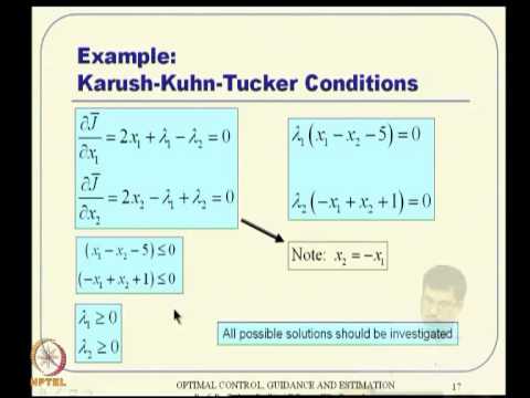
So, what it tells us? It gives us these two conditions. That means, del j by del x i is
to be equal to 0 and lambda j g j has to be equal to 0. These are the two equations, so
using which we have to solve for various conditions for lambdas and all that actually. Then, for
for j of x is
…