en English
Untitled English subtitles
Report a problem
Advertisement
English transcript
PATRICK WINSTON: Here we are, partway into our discussion of
how it might be possible to make a
computer learn something.
Now let's face it, we're pretty good at learning.
And on top of that, if you remove the skull, all you find
is neurons in there.
Our heads are stuffed with them.
So it would seem that if we're to make a smart computer, one
that could learn something, we ought to think
about mimicking biology.
And a great deal of effort has gone into mimicking
neurobiology over the years, and today I want to
tell you about it.
So by the end of the hour, you'll know how to construct
your own neural net, and you'll know how to criticize
someone who offers to sell you a magic box that uses a neural
net to predict something.
So first of all, let's look a little bit of naive biology,
and reflect a little bit on what neurons are like.
There are lots of different kinds, but this is naive
neurobiology, so we're just going to talk about the
standard kind.
And like all cells, there's a cell body
with a nucleus inside.
But in contrast to most cells, there's typically a long
protrusion called an axon.
And an axon divides in two relatively infrequently.
But sometimes they do divide.
That division is called a bifurcation, because it's a
division into two parts.
On the other end of the neuron, you have a whole lot
of things that branch off, like so.
And these things, in contrast to the axon, do nothing but
branch like crazy, in general.
And that part of the axon, that part of the neuron is
called the dendritic tree.
And so the dendritic tree creates a huge number of
places that downstream axons can connect to.
So a downstream axon, it's the business end of a neuron.
Off there, out the door.
It might come in and find a place on the dendritic tree
with which it wants to connect.
Now it isn't quite that simple, because the nature of
the connection is such that that downstream axon--
it's a little bulb on the end.
And there is a little space between that downstream axon
and this upstream dendrite.
This is filled with little vesicles, the
neurotransmitters that get dumped into
that synaptic space.
And when there's dumping of the vesicles into the synaptic
space, it excites the dendrite.
And if there's enough cumulative excitement on the
dendritic tree, then what happens is that a single spike
propagates down the axon.
So that's a little naive biology, and there's some
aspects of it that we should right away take note of.
Number one, there are the synapses.
And some of these synapses are thought to be more important
than others.
That is to say, they exert more influence on the
performance of the neuron.
So we have the notion of synaptic weights.
Some of them have a higher influence or higher weight
than others.
Then the next thing we need to take note of is a sort of
cumulative effect.
Cumulative.
That is to say, all that stuff that's coming in on the
dendritic tree is somehow added up or combined or put
together with some function.
Who knows what it is, but there's a kind of accumulation
of stimulation on this dendritic tree, which leads to
a decision about whether that spike goes down the axon.
It either does or it doesn't, so there's a certain all or
none phenomenon here, which is another way of saying that the
spike either goes or it doesn't go.
And those are three handy observations.
Those are three knee-jerk observations.
There's a lot, lot, lot more you could say about
what goes on there.
In fact, you could take a whole complicated course on
what goes on in a single neuron.
And you'll talk about sodium and potassium and gradients
and refractory periods and all that sort of stuff.
But this is all we're going to do.
It's the only thing we're going to take note of today.
These kinds of characteristics.
And now we're going to do is say, OK, given those kinds of
characteristics, how do we make a model of it?
Because this is MIT, after all.
We make models of everything.
That's what MIT is all about.
So let's make a model of this little biological element.
Well, let's see.
First thing we're going to do is, we're going
to have some inputs.
Input one, and it's going to come into a multiplier and get
multiplied by some weight, weights of one.
And then we might have lots of inputs.
Input n would get multiplied times some weight n.
Like so.
Well, what have we done so far?
Well, we've got number one modeled.
That's that part there.
Next thing we have to do is, we have to have some way of
combining all these influences, all these products
of the weights times the strength of the input.
So we're going to do is, we're going to run all those guys
into a summation box.
So there's a real big modeling decision that we made.
We're going to just take the sum of the inputs.
And there might be many of those, so let me draw a few
more arrows here.
Next thing need to do, though, is we have to say, well the
output is not proportional to the input, but rather it's an
all or none kind of phenomenon.
So we're going to have to run the output of the summer
through a thresholding box.
So here's the function that's performed by the
thresholding box.
It's going to be zero output until we get the sum
threshold, and then we're going to put out a one.
So the output here is either going to be zero or one.
So we might as well say since that's going to be input to
the neurons downstream, that the inputs are also zero one--
either zero or one.
So now we have a model of a neuron.
It's a naive model.
It doesn't take into account much about what
real neurons are like.
Nevertheless, it is a model, and we can ask what
we can do with it.
Of course, one thing we could do with it is we could put a
whole bunch of these together in a big can and stir it up
and see what happens.
So there'll be some elements here.
There would be some neurons in here.
And some of them will take an input from the outside.
There's x1.
Here's xn.
And it goes in here and finds some other
multiplier, and so on.
And then there'll be some summation boxes, and there'll
be these weights.
There'll be other weights.
And then there'll be these threshold boxes, which I made
look like that, and they will produce some
outputs for this system.
Like so.
And we'll call these outputs z1 through zm, having
already used up n.
So there it is.
There's a neural net, abstractly speaking.
But nevertheless, it's enough of a notion that we can now
say that the output vector--
that's an output vector, right?
There are a whole bunch of zs.
The output vector is equal to some vector function of the
inputs x and what else?
Well, the weights, right?
It will depend on the weights.
It also depends a whole lot on the structure, but for a fixed
structure, fixed way of arranging the neurons, all
that the output can possibly depend on is the input and
those weights.
So that's z--
the output.
Now of course, if we have some training samples, then we have
some desired outputs for particular inputs.
We can write that down, too.
We can say that the desired output, d, also vector, is
equal to some function.
Now we don't care about the weights.
We just want a particular output given
a particular input.
So that's going to be some function of g, some
function g of x.
And now the neural net problem is easily stated.
We want to bring f of x into alignment with g of x.
That is to say, we want a set of weights that make the
actual output the same as the output that we desire.
So that's simple, right?
At least abstractly.
It's a simple idea.
Yeah, it's simple.
Why don't we just go home?
Well, first of all, we need a few things.
Number one, we need to know how bad we're doing.
Or if you're a more optimistic type, how well we're doing.
So we need some measure of how good our set of weights is.
And that must be a function of the difference or must be some
function of the desired outputs and the actual
outputs, right?
So we need a performance function.
Just for fun, we'll call it p.
So p is a function of the desired outputs and the actual
outputs, like so.
And the one we're going to use today is this one.
We're going to say that the performance is equal to, I
don't know, d minus z, the difference.
Let's take the magnitude of that, and let's multiply it by
1/2, and let's square it.
Where the devil did that come from?
Did God say that's the right way to do it?
You don't think so, Leonardo?
Why don't I make that the performance function?
LEONARDO: You wanted to minimize the distance squared,
and you're normalizing-- you're trying to minimize the
distance to a line.
PATRICK WINSTON: So did God say this is the best
performance function to use?
It turns out to be.
A little more than adequate.
It turns out to be good.
It turns out to be mathematically convenient to
use this particular metric.
And that's not a bad thing to have.
After all, if we draw a graph of this, there's only one d
and one z, so it isn't a vector, that the
graph looks like this.
So we'd like to minimize that quantity.
There must be some imprinting early in 1801, because I don't
like to think about minimizing stuff.
I like to think about maximizing stuff.
So we're not actually going to use this as
our performance function.
We're going to use this as our performance function.
We'll put a minus sign in front, so that the
curve looks like that.
And what we're trying to do then is, we're trying to
maximize that performance function.
It can only be negative.
We're trying to maximize it.
When it's at maximum, it's zero.
It just the difference between going uphill going downhill.
I like to think about going uphill.
Well, now we're on our way.
All we have to do is find some way of finding the best
combination of W's that do the right thing to that
performance function.
So let's have a look at the world's simplest situation,
where we just have two weights in there, W1 and W2.
Now for those of you who climb mountains and stuff, you'll
recognize that I'm going to draw a little topographic map
of the performance function.
And I'm going to assume that it looks like that.
These are [? equi ?] performance lines.
And now suppose that we start off with some combination of
W1 and W2 handed to us by a random number generator, say.
And let's say that we start off right there.
Now we've already had a good part of 6034, so we know what
to do, right?
My god, I've even talked about mountains.
It's a hill climbing problem.
So we can do what we learned about real
early in the subject.
We could do a hill-climbing type depth
first search type thing.
And if we do that, what we do is we say, well, I could
either move north.
I could move west.
I could move south.
Or I could move east.
And plainly, east is the winner, because
that's taking us uphill.
So if that were all our work, this, then we could all go
home and sleep.
But it isn't.
We can sleep anyway, I guess.
Come to think of it.
But this isn't all there is to it, because the trouble is, if
there are lots of W's, this becomes a hugely high
dimensional space.
So this idea of trying one move in each direction doesn't
work very well.
So we have to think of something better to do.
By the way, nevertheless, this is the--
wait a second.
Halt.
We forgot that we don't have any thresholds in here,
either, in our model.
So we need to have some way of altering not only the weights,
but I guess, come to think of it, up in here we can have
thresholds that we can adjust as well.
But there's a trick that will enable us to get rid of
thinking about the thresholds.
So let me tell you about that trick.
What we're going to do is, we're going to add an extra
input here, like this.
It's going to have a multiplier on it like this.
It's going to be permanently connected to -1.
And it's going to have a weight coming in on W0.
So we got W0, W1, through Wn, and what we're going to do is,
we're going to make W0 equal to that threshold.
And if we do that, that's subtracts t off of this thing.
So instead of firing at t, we ought to fire at zero.
So what we're going to do then is, we're going to replace our
original threshold function with one that looks like this.
Same thing, only it triggers at zero.
But now you see we've rendered that thing as a weight, and we
can adjust that weight just like any other ones.
We can hill climb or whatever we want to do.
So we've got a series of tricks here, and let's call
this trick number one.
Now over here, we've decided that ordinary hill climbing
won't help much because are too many dimensions.
But we've all taken 1802 or something like that, and we
know what to do with a situation like this, where
we're trying to climb around in some space and we're trying
to find the highest place we can get to.
We know what to do, right?
We have the method of--
what do you think, Casey?
CASEY: [INAUDIBLE].
PATRICK WINSTON: You do what?
Yeah, you go up perpendicular to the contour line using the
method of what?
Gradient?
Now there's only two possibilities--
ascent or descent.
And I've arranged to go up, so this is gradient ascent.
We're trying to cross those contour lines perpendicularly,
so we've got gradient descent.
So instead of just trying out these northeast, southwest
deals, what we can do is we can try
to go in that direction.
And to go in that direction, we could just use good old
180-something-or-other and say that delta W, the difference
in the weights that we want to use, is equal to-- let's take
the partial derivative of the performance
function in the x direction.
Multiply that times a little vector I in that direction.
Plus the partial of the performance function with
respect to y, plus a unit vector in the up direction.
And so that becomes our delta W. Except that maybe we want
to put a little rate constant up there, like so.
So that's the rate constant.
Now let's see if this makes sense.
We want to make sure that the math makes sense intuitively.
If I go in this direction, and if that partial derivative is
big, that means I'm getting a lot of bang for my x buck.
And so that sounds good.
I want to go a lot in that direction.
On the other hand, if I'm not getting very much out of going
in the y direction, as I am not here, that means that the
partial derivative will be small.
That means I don't want to go much in that direction.
I want to go mostly in the x direction, and only little bit
in the y direction.
And that's what it says here.
This partials big.
This partial's small.
So I'm going to end up going in that direction.
In fact, my arrow's a little bit too
severely in that direction.
It's probably more like that, crossing the
local contour line.
So that's what we're going to do.
We're going to use gradient ascent.
Except that we can't use gradient ascent.
There's something about our problem that isn't like what
we had an 180-something-or-other.
What's the problem?
Well, what is required before you can use gradient ascent?
LEONARDO: [INAUDIBLE].
PATRICK WINSTON: Leonardo says we have to have a smooth,
continuous function.
And this is anything but smooth, because we got that
step function in there.
So this method won't work.
But anyhow, this is a good idea, and we'll call this
insight number two.
But wait a second.
We can fix this, actually, because we God didn't say we
had to use a step function.
We could use a smooth function.
So why don't we come back over here and then make yet another
adjustment?
We've got that, but we want to adjust it again.
And what we want to do is we want to have a threshold
function that's not sharp like that, but rather
on the smooth side.
Let's use all of our colors while we've got them.
So maybe what we want to do is have something that is the
same on the ends, but which is a little bit
smoother in going through.
Zero looks like that.
That would certainly do the job for us, and in fact, the
function we're going to use is 1 over 1 plus e to the minus
alpha, where this is alpha.
Now, did God say that was the right-- it does have that
shape, right?
So if alpha is very large, then e to the
minus alpha is 0.
Then it's 1.
On the other hand, if alpha is very negative, then it's 1
plus some big number-- that's 0.
And if alpha is equal to 0, then it's 1 plus 1, so that's
1/2, just like I drew it.
But there are a lot of functions
that have that property.
So why did I use this one?
Did God say I should use this one?
But it might turn out to be--
SPEAKER 1: The simplest or the best.
PATRICK WINSTON: Why would it be the best?
Because it's mathematically convenient.
Yeah, that's right.
Maybe it'll turn out to be mathematically convenient.
That's insight number one, that's insight number two, and
this is insight number three.
And impossible problems are often solved we have three
insights in a row.
And this one is in fact solved when we have three of those
insights in a row.
So now I could just write down the formula, and you'll see
the formula in other venues, but I refuse to do it.
Because what I want to do is, I want to work my way through
the world simplest neural net that illustrates
the necessary ideas.
So here's what the world's simplest
neural net looks like.
The input-- there's just one input, x.
It's multiplied times some weight, W1, and that produces
a product, P1.
And that goes into a threshold box, which is this function
here which looks like this curve here.
And since it looks like an S, we're going to call that a
sigmoid function.
It's a sigmoid function.
Did you ever hear about a sigmoid function before in
this course?
It's exactly what we use as our thresholds on quiz grades.
So we're going to use a curve that looks like that.
And then out here comes y.
And then y is multiplied by another weight, W2.
And that produces P2.
And that goes into another sigmoid, like so,
and produces z.
And z goes into the performance calculating box.
And out here comes P, which is equal to -1/2 the desired
output minus the actual output squared.
And now since I've only got one thing and not a vector, I
write it as a scalar.
So what I'm assuming is that I have some samples
with desired values.
And I can observe z, the actual values.
And I want to bring them into conformity by doing these
partial derivatives and stuff and then making the necessary
adjustments to the weights.
Simple, right?
Now this is where I got to do a little partial
differentiation and stuff, so you down here in front and in
charge of making sure I don't make any mistakes.
And if I make any mistakes, we'll all hold you
accountable.
So I don't know what to do with that, actually.
What a mess.
Well, let's see.
According to the formula on the middle board--
let me forget the rate constant.
We can put that back in later.
But according to that thing there, I need to calculate in
order to figure out how much of a change to make to these
W's, I have to calculate the partial derivatives of that
performance function.
And jeez, I better make an adjustment here
before it's too late.
X is actually W1 of my diagram, and y is actually W2
in my diagram.
So what I want to do is I want to calculate those partial
derivatives.
So I have a partial of the performance function with
respect to W1.
Anybody work that out in our head?
Oops, wait a minute.
What have I done?
Sorry, W2 here.
Let's start with W2, since it's closer to the output.
Partial of the performance function P with respect to W2.
How do I do that?
I could throw up my hands and give up, but no.
I went to MIT, too, and know about 1801 stuff, and I know
in particular about what?
When you want to compute a derivative and there's a whole
bunch of junk in the way.
Gosh, I feel all tied pu.
I feel like I am shackled by what?
SPEAKER 2: The chain rule.
PATRICK WINSTON: The chain rule!
Thank you.
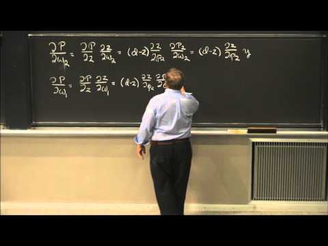
OK, so the partial of P with respect to W2 can be written
as the partial of P with respect to z times the partial
of z with respect to W2.
Well, here's P and here's z , so I can take the partial
derivative of that pretty straightforwardly.
Let's see.
I bring the 2 down.
That cancels with the 1/2.
Then I've got d minus c.
Then I take the derivative of the insides, which is -1,
which cancels my -1 out here.
Oh, I think we can do that in our head.
Tha
…