en English
Untitled English subtitles
Report a problem
Advertisement
English transcript
PATRICK WINSTON: So where are we?
We started off with simple methods for learning stuff.
Then, we talked a little about a purchase of learning that
we're vaguely inspired by.
The fact that our heads are stuffed with neurons, and that
we seemed to have evolved from primates.
Then, we talked about looking at the problem and address the
issue of [? phrenology ?]
and how it's possible to learn concepts.
But now, we're coming full circle back to the beginning
and thinking about how to divide up a space with
decision boundaries.
But whereas, you do it with a neural net or a nearest
neighbors or a ID tree.
Those are very simple ideas that work very often.
Today, we're going to talk about a very sophisticated
idea that still has a implementation.
So this needs to be in the tool bag of
every civilized person.
This is about support vector machines, an
idea that was developed.
Well, I want to talk to you today about how
ideas develop, actually.
Because you look at stuff like this in a book, and you think,
well, Vladimir Vapnik just figured this out one Saturday
afternoon when the weather was too bad to go outside.
That's not how it happens.
It happens very differently.
I want to talk to you a little about that.
The next thing about great things that were done by
people who are still alive is you can ask them
how they did it.
You can't do that with Fourier.
You can't say to Fourier, how did you do it?
Did you dream it up on a Saturday afternoon?
But can call Vapnik on the phone and ask him questions.
That's the stuff I'm going to talk about toward
the end of the hour.
Well, it's all about decision boundaries.
And now, we have several techniques that we can use to
draw some decision boundaries.
And here's the same problem.
And if we drew decision boundaries in here, we might
get something that would look like maybe this.
If we were doing a nearest neighbor approach, and if
we're doing ID trees, we'll just draw in a line like that.
And if we're doing neural nets, well, you can put in a
lot of straight lines wherever you like with a neural net,
depending on how it's trained up.
Or if you just simply go in there and design it, so you
could do that if you wanted.
And you would think that after people have been working on
this sort of stuff for 50 or 75 years that there wouldn't
be any tricks in the bag left.
And that's when everybody got surprised, because around the
early '90s Vladimir Vapnik introduced the ideas I'm about
to talk to you about.
So what Vapnik says is something like this.
Here you have a space, and you have some negative examples,
and you have some positive examples.
How do you divide the positive examples from
the negative examples?
And what he says that we want to do is we want to draw a
straight line.
But which straight line is the question.
Well, we want to draw a straight line.
Well, would this be a good straight line?
One that went up like that?
Probably not so hot.
How about one that's just right here?
Well, that might separate them, but it seems awfully
close to the negative examples.
So maybe what we ought to do is we ought to draw our
straight line in here, sort of like this.
And that line is drawn with a view toward putting in the
widest street that separates the positive samples from the
negative samples.
That's why I call it the widest street approach.
So that makes way of putting in the decision boundary--
is to put in a straight line but in contrast with the way
ID tree puts in a straight line.
It tries to put the line in in such a way as the separation
between the positive and negative examples.
That street is as wide as possible.
All right.
So you might think to do that in the UROP project, and then,
let it go with that.
What's the big deal?
So what we've got to do is we've got to go through why
it's a big deal.
So first of all, we like to think about how you would make
a decision rule that would use that decision boundary.
So what I'm going to ask you to imagine is that we've got a
vector of any length that you like, constrained to be
perpendicular to the median, or if you like, perpendicular
to the gutters.
It's perpendicular to the median line of the street.
All right, it's drawn in such a way that that's true.
We don't know anything about it's length, yet.
Then, we also have some unknown, say, right here.
And we have a vector that points to it by excel.
So now, what we're really interested in is whether or
not that unknown is on the right side of the street or on
the left side of the street.
So what we'd what to do is want to project that vector,
u, down on to one that's perpendicular to the street.
Because then, we'll have the distance in this direction or
a number that's proportional to this in this direction.
And the further out we go, the closer we'll get to being on
the right side of the street, where the right side of the
street is not the correct side but actually the right side of
the street.
So what we can do is we can say, let's take w and dot it
with u and measure whether or not that number is equal to or
greater than some constant, c.
So remember that the dot product has taken the
projection onto w.
And the bigger that projection is, the further out along this
line the projection will lie.
And eventually it will be so big that the projection
crosses the median line of the street, and we'll say it must
be a positive sample.
Or we could say, without loss of generality that the dot
product plus some constant, b, is equal to or greater than 0.
If that's true, then it's a positive sample.
So that's our decision rule.
And this is the first in several elements that we're
going to have to line up to understand this idea called
support vector machines.
So that's the decision rule.
And the trouble is we don't know what constant to use, and
we don't know which w to use either.
We know that w has to be perpendicular to the median
line of the street.
But there's lot of w's that are perpendicular to the
median line of the street, because it
could be of any length.
So we don't have enough constraint here to fix a
particular b or a particular w.
Are you with me so far?
All right.
And this, by the way, we get just by saying that c
equals minus b.
What we're going to do next is we're going to lay on some
additional constraints whether you're toward putting enough
constraint on the situation that we can actually calculate
a b and a w.
So what we're going to say is this, that if we look at this
quantity that we're checking out to be greater than or less
than 0 to make our decision, then, what we're going to do
is we're going to say that if we take that vector w, and we
take the dot product of that with some x plus, some
positive sample, now.
This is not an unknown.
This is a positive sample.
If we take the dot product of those two vectors, and we had
b just like in our decision rule, we're going to want that
to be equal to or greater than 1.
So in other words, you can be an unknown anywhere in this
street and be just a little bit greater or just a little
bit less than 0.
But if you're a positive sample, we're going to insist
that this decision function gives the
value of one or greater.
Likewise, if w thought it was some negative sample is
provided to us, then we're going to say that has to be
equal to or less than minus 1.
All right.
So if you're a minus sample, like one of these two guys or
any minus sample that may lie down here, this function that
gives us the decision rule must return minus 1 or less.
So there's a separation of distance here.
Minus 1 to plus 1 for all of the samples.
So that's cool.
But we're not quite done, because carrying around two
equations like this, it's a pain.
So what we're going to do is we're going to introduce
another variable to make like a little easier.
Like many things that we do, and when we develop this kind
of stuff, introducing this variable is not something that
God says has to be done.
What is it?
We introduced this additional stuff to do what?
To make the mathematics more convenient, so mathematical
convenience.
So what we're going to do is we're going to introduce a
variable, y sub i, such that y sub i is equal to plus 1 for
plus samples and minus 1 for negative samples.
All right.
So for each sample, we're going to have a value for this
new quantity we've introduced, y.
And the value of y is going to be determined by whether it's
a positive sample or negative sample.
If it's a positive sample it's got to be plus 1 for this
situation up here, and it's going to be minus 1 for this
situation down here.
So what we're going to do with this first equation is we're
going to multiply it by y sub i, and that is now x of i,
plus b is equal to or greater than 1.
And then, you know what we're going to do?
We're going to multiply the left side of this equation by
y sub i, as well.
So the second equation becomes y sub i times x sub i plus b.
And now, what does that do over here?
We multiplied this guy times minus 1.
So it used to be the case that that was less than minus 1.
So if we multiply it by minus 1, then it has to be greater
than plus 1.
The two equations are the same, because that introduces
this little mathematical convenience.
So now, we can say that y sub i times x sub i plus b.
Well, what we're going to do--
Brett?
STUDENT: What happened to the w?
PATRICK WINSTON: Oh, did I leave out a w?
I'm sorry.
Thank you.
Yeah, I wouldn't have gotten very far with that.
So that's dot it with w, dot it with w.
Thank you, Brett.
Those are all vectors.
I'll pretty soon forget to put the little vector marks on
there, but you know what I mean.
So that's w plus b.
And now, let me bring that 1 over to the left side, and
that's equal to or greater than 0.
All right.
With Brett's correction, I think everything's OK.
But we're going to take one more step, and we're going to
say that y sub i times x sub i times w plus b minus 1.
It's always got to be equal to or greater than 0.
But what I'm going to say is if we're for
x sub i in a gutter.
So there's always going to be greater than 0, but we're
going to add the additional constraint that it's going to
be exactly 0 for all the samples that end up in the
gutters here of the street.
So the value of that expression is going to be
exactly 0 for that sample, 0 for this sample and this
sample, not 0 for that sample.
It's got to be greater than 1.
All right?
So that's step number two.
And this is step number one.
OK.
So now, we've just got some expressions to talk about,
some constraints.
Now, what are we trying to do here?
I forgot.
Oh, I remember now.
We're trying to figure out how to arrange for the line to be
such at the street separating the pluses from the minuses as
wide as possible.
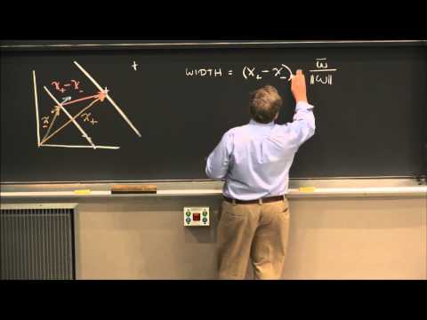
So maybe we better figure out how we can express the
distance between the two gutters.
Let's just repeat our drawing.
We've got some minuses here, got pluses out here, and we've
got gutters that are going down here.
And now, we've got a vector here to a minus, and we've got
a vector here to a plus.
So we'll call that x plus and this x minus.
So what's the width of the street?
I don't know, yet.
But what we can do is we can take the difference of those
two vectors, and that will be a vector that
looks like this, right?
So that's x plus minus x minus.
So now, if I only had a unit normal that's normal to the
median line of the street, if it's a unit normal, then I
could just take the dot product or that unit normal
and this difference vector, and that would be the width of
the street, right?
So in other words, if I had a unit vector in that direction,
then I could just dot the two together, and that would be
the width of the street.
So let me write that down before I forget.
So the width is equal to x plus minus x minus.
OK.
That's the difference vector.
And now, I've got to multiple it by unit vector.
But wait a minute.
I said that that w is a normal, right?
The w is a normal.
So what I can do is I can multiply this times w, and
then, we'll divide by the magnitude of w, and that will
make it a unit vector.
So that dot product, not a product, that dot product is,
in fact, a scalar, and it's the width of the street.
It doesn't do as much good, because it doesn't look like
we get much out of it.
Oh, but I don't know.
Let's see, what can we get out of it?
Oh gee, we've got this equation over here, this
equation that constrains the samples
that lie in the gutter.
So if we have a positive sample, for example, then this
is plus 1, and we have this equation.
So it says that x plus times w is equal to, oh, 1 minus b.
See, I'm just taking this part here, this vector here, and
I'm dotting it with x plus.
So that's this piece right here.
y is 1 for this kind of sample.
So I'll just take the 1 and the b back over to the other
side, and I've got 1 minus b.
OK?
Well, we can do the same trick with x minus.
If we've got a negative sample,
then y sub i is negative.
That gives us our negative w times dot over x sub i.
But now, we take this stuff back over to the right side,
and we get 1 plus b.
So that all licenses to rewrite this thing as 2 over
the magnitude of w.
How did I get there?
Well, I decided I was going to enforce this constraint.
I noted that the width of the street has got to be this
difference vector times a unit vector.
Then, I used the constraint to plug back some values here.
And I discovered to my delight and amazement that the width
of the street is 2 over the magnitude of w.
Yes, Brett?
STUDENT: So your first x plus is minus b, and x
minus is 1 plus b.
PATRICK WINSTON: Yeah.
STUDENT: So you're subtracting it?
PATRICK WINSTON: Let's see.
If I've got a minus here, then that makes that minus, and
then, the b is minus, and when I take the b over to the other
side it becomes plus.
STUDENT: Yeah, so if you subtract the left with the
right [INAUDIBLE].
PATRICK WINSTON: No.
No, sorry.
This expression here is 1 plus b.
Trust me it works.
I haven't got my legs all tangled up like last Friday,
well, not yet, anyway.
It's possible.
There's going to be a lot of algebra here eventually.
So this quantity here, this is miracle number three.
This quantity here is the width of the street.
And what we're trying to do is we're trying to
maximize that, right?
So we want to maximize 2 over the magnitude of w if we're to
get the widest street under the constraints that we've
decided that we're going to work with.
All right.
So that means that it's OK to maximize 1 over w, instead.
We just drop the constant.
And that means that it's OK to minimize the
magnitude of w, right?
And that means that it's OK to minimize 1/2 times the
magnitude of w squared.
Right, Brett?
Why did I do that?
Why did I multiply by 1/2 and square it?
STUDENT: Because it's mathematically convenient.
PATRICK WINSTON: It's mathematically convenient.
Thank you.
So this is point number three in the development.
So where do we go?
We decided that was going to be our decision rule.
We're going to see which side of the line we're on.
We decided to constrain the situation, so the value of the
decision rule is plus 1 in the gutters for the positive
samples and minus 1 in the gutters for
the negative samples.
And then, we discovered that maximizing the width of the
street led us to an expression like that,
which we wish to maximize.
Should we take a break?
Should we get coffee?
Too bad, we can't do that in this kind of situation.
But we would if we could.
And I'm sure when Vapnik got to this point, he
went out for coffee.
So now, we back up, and we say, well, let's let these
expressions start developing into a song.
Not like that, that's vapid, speaking of Vapnik.
What song is it going to sing?
We've got an expression here that we'd like to find the
minimum of, the extremum of.
And we've got some constraints here that we
would like to honor.
What are we going to do?
Let me put what we're going to do to you in
the form of a puzzle.
Is it got something to do with Legendre?
Has it got something to do with Laplace?
Or does it have something to do with Lagrange?
She says Lagrange.
Actually, all three were said to be on Fourier's Doctoral
Defense Committee-- must have been quite an example.
But we want to talk about Lagrange, because we've got a
situation here.
Is this 1801?
1802?
1802.
We learned in 1802 that if we going to find the extremum of
a function with constraints, then we're going to have to
use Lagrange multipliers.
That would give us a new expression, which we can
maximize or minimize without thinking about
the constraints anymore.
That's how Lagrange multipliers work.
So this brings us to miracle number four, developmental
piece number four.
And it works like this.
We're going to say that L--
the thing we're going to try to maximize in order to
maximize the width of the street--
is equal to 1/2 times the magnitude of that vector, w,
squared minus.
And now, we've got to have a summation over all the
constraints.
And each or those constraints is going to have a multiplier,
alpha sub i.
And then, we write down the constraint.
And when we write down a constraint,
there it is up there.
And I've got to be hyper careful here, because,
otherwise, I'll get lost in the algebra.
So the constraint is y sub i times vector, w, dotted with
vector x sub i plus b, and now, I've got a closing
parenthesis, a minus 1.
That's the end of my constraint, like so.
I sure hope I've got that right, because I'll be in deep
trouble if that's wrong.
Anybody see any bugs in that?
That looks right. doesn't it?
We've got the original thing we're trying to work with.
Now, we've got Lagrange multipliers all multiplied.
It's back to that constraint up there, where each
constraint is constrained to be 0.
Well, there's a little bit of mathematical slight of hand
here, because in the end, the ones that are going to be 0,
the Lagrange multipliers here.
The ones that are going to be non 0 are going to be the ones
connected with vectors that lie in the gutter.
The rest are going to be 0.
But in any event, we can pretend that this is what
we're doing.
I don't care whether it's a maximum or minimum.
I've lost track.
But what we're going to do is we're going to try to find an
extremum of that.
So what do we do?
What does 1801 teach us about?
Finding the maximum--
well, we've got to find the derivatives and set them to 0.
And then, after we've done that, a little bit of that
manipulation, we're going to see a wonderful
song start to emerge.
So let's see if we can do it.
Let's take the partial of L, the Lagrangian, with respect
to the vector, w.
Oh my God, how do you differentiate with
respect to a vector?
It turns out that it has a form that looks exactly like
differentiating with respect to a scalar.
And the way you prove that to yourself is you just expand
everything in terms of all of the vector's components.
You differentiate those with respect to what you're
differentiating with respect to, and everything
turns out the same.
So what you get when you differentiate this with
respect to the vector, w, is 2 comes down, and we have just
magnitude of w.
Was it the magnitude of w?
Yeah, like so.
Was it the magnitude of w?
Oh, it's not the magnitude of w.
It's just w, like so, no magnitude involved.
Then, we've got a w over here, so we've got to differentiate
this part with respect to w, as well.
But that part's a lot easier, because all we
have there is a w.
There's no magnitude.
It's not raised to any power.
So what's w multiplied by?
Well, it's multiplied by x and y sub i and alpha sub i.
All right.
So that means that this expression, this derivative of
the Lagrangian, with respect to w is going to be equal to w
minus the sum of alpha sub i, y sub i, x sub i, and that's
got to be set to 0.
And that implies that w is equal to the sum of some alpha
i, some scalars, times this minus 1 or plus 1 variable
times x sub i over i.
And now, the math is beginning to sing.
Because it tells us that the vector w is a linear sum of
the samples, all the samples or some of the sample.
It didn't have to be that way.
It could have been raised to a power.
It could have b
…
We started off with simple methods for learning stuff.
Then, we talked a little about a purchase of learning that
we're vaguely inspired by.
The fact that our heads are stuffed with neurons, and that
we seemed to have evolved from primates.
Then, we talked about looking at the problem and address the
issue of [? phrenology ?]
and how it's possible to learn concepts.
But now, we're coming full circle back to the beginning
and thinking about how to divide up a space with
decision boundaries.
But whereas, you do it with a neural net or a nearest
neighbors or a ID tree.
Those are very simple ideas that work very often.
Today, we're going to talk about a very sophisticated
idea that still has a implementation.
So this needs to be in the tool bag of
every civilized person.
This is about support vector machines, an
idea that was developed.
Well, I want to talk to you today about how
ideas develop, actually.
Because you look at stuff like this in a book, and you think,
well, Vladimir Vapnik just figured this out one Saturday
afternoon when the weather was too bad to go outside.
That's not how it happens.
It happens very differently.
I want to talk to you a little about that.
The next thing about great things that were done by
people who are still alive is you can ask them
how they did it.
You can't do that with Fourier.
You can't say to Fourier, how did you do it?
Did you dream it up on a Saturday afternoon?
But can call Vapnik on the phone and ask him questions.
That's the stuff I'm going to talk about toward
the end of the hour.
Well, it's all about decision boundaries.
And now, we have several techniques that we can use to
draw some decision boundaries.
And here's the same problem.
And if we drew decision boundaries in here, we might
get something that would look like maybe this.
If we were doing a nearest neighbor approach, and if
we're doing ID trees, we'll just draw in a line like that.
And if we're doing neural nets, well, you can put in a
lot of straight lines wherever you like with a neural net,
depending on how it's trained up.
Or if you just simply go in there and design it, so you
could do that if you wanted.
And you would think that after people have been working on
this sort of stuff for 50 or 75 years that there wouldn't
be any tricks in the bag left.
And that's when everybody got surprised, because around the
early '90s Vladimir Vapnik introduced the ideas I'm about
to talk to you about.
So what Vapnik says is something like this.
Here you have a space, and you have some negative examples,
and you have some positive examples.
How do you divide the positive examples from
the negative examples?
And what he says that we want to do is we want to draw a
straight line.
But which straight line is the question.
Well, we want to draw a straight line.
Well, would this be a good straight line?
One that went up like that?
Probably not so hot.
How about one that's just right here?
Well, that might separate them, but it seems awfully
close to the negative examples.
So maybe what we ought to do is we ought to draw our
straight line in here, sort of like this.
And that line is drawn with a view toward putting in the
widest street that separates the positive samples from the
negative samples.
That's why I call it the widest street approach.
So that makes way of putting in the decision boundary--
is to put in a straight line but in contrast with the way
ID tree puts in a straight line.
It tries to put the line in in such a way as the separation
between the positive and negative examples.
That street is as wide as possible.
All right.
So you might think to do that in the UROP project, and then,
let it go with that.
What's the big deal?
So what we've got to do is we've got to go through why
it's a big deal.
So first of all, we like to think about how you would make
a decision rule that would use that decision boundary.
So what I'm going to ask you to imagine is that we've got a
vector of any length that you like, constrained to be
perpendicular to the median, or if you like, perpendicular
to the gutters.
It's perpendicular to the median line of the street.
All right, it's drawn in such a way that that's true.
We don't know anything about it's length, yet.
Then, we also have some unknown, say, right here.
And we have a vector that points to it by excel.
So now, what we're really interested in is whether or
not that unknown is on the right side of the street or on
the left side of the street.
So what we'd what to do is want to project that vector,
u, down on to one that's perpendicular to the street.
Because then, we'll have the distance in this direction or
a number that's proportional to this in this direction.
And the further out we go, the closer we'll get to being on
the right side of the street, where the right side of the
street is not the correct side but actually the right side of
the street.
So what we can do is we can say, let's take w and dot it
with u and measure whether or not that number is equal to or
greater than some constant, c.
So remember that the dot product has taken the
projection onto w.
And the bigger that projection is, the further out along this
line the projection will lie.
And eventually it will be so big that the projection
crosses the median line of the street, and we'll say it must
be a positive sample.
Or we could say, without loss of generality that the dot
product plus some constant, b, is equal to or greater than 0.
If that's true, then it's a positive sample.
So that's our decision rule.
And this is the first in several elements that we're
going to have to line up to understand this idea called
support vector machines.
So that's the decision rule.
And the trouble is we don't know what constant to use, and
we don't know which w to use either.
We know that w has to be perpendicular to the median
line of the street.
But there's lot of w's that are perpendicular to the
median line of the street, because it
could be of any length.
So we don't have enough constraint here to fix a
particular b or a particular w.
Are you with me so far?
All right.
And this, by the way, we get just by saying that c
equals minus b.
What we're going to do next is we're going to lay on some
additional constraints whether you're toward putting enough
constraint on the situation that we can actually calculate
a b and a w.
So what we're going to say is this, that if we look at this
quantity that we're checking out to be greater than or less
than 0 to make our decision, then, what we're going to do
is we're going to say that if we take that vector w, and we
take the dot product of that with some x plus, some
positive sample, now.
This is not an unknown.
This is a positive sample.
If we take the dot product of those two vectors, and we had
b just like in our decision rule, we're going to want that
to be equal to or greater than 1.
So in other words, you can be an unknown anywhere in this
street and be just a little bit greater or just a little
bit less than 0.
But if you're a positive sample, we're going to insist
that this decision function gives the
value of one or greater.
Likewise, if w thought it was some negative sample is
provided to us, then we're going to say that has to be
equal to or less than minus 1.
All right.
So if you're a minus sample, like one of these two guys or
any minus sample that may lie down here, this function that
gives us the decision rule must return minus 1 or less.
So there's a separation of distance here.
Minus 1 to plus 1 for all of the samples.
So that's cool.
But we're not quite done, because carrying around two
equations like this, it's a pain.
So what we're going to do is we're going to introduce
another variable to make like a little easier.
Like many things that we do, and when we develop this kind
of stuff, introducing this variable is not something that
God says has to be done.
What is it?
We introduced this additional stuff to do what?
To make the mathematics more convenient, so mathematical
convenience.
So what we're going to do is we're going to introduce a
variable, y sub i, such that y sub i is equal to plus 1 for
plus samples and minus 1 for negative samples.
All right.
So for each sample, we're going to have a value for this
new quantity we've introduced, y.
And the value of y is going to be determined by whether it's
a positive sample or negative sample.
If it's a positive sample it's got to be plus 1 for this
situation up here, and it's going to be minus 1 for this
situation down here.
So what we're going to do with this first equation is we're
going to multiply it by y sub i, and that is now x of i,
plus b is equal to or greater than 1.
And then, you know what we're going to do?
We're going to multiply the left side of this equation by
y sub i, as well.
So the second equation becomes y sub i times x sub i plus b.
And now, what does that do over here?
We multiplied this guy times minus 1.
So it used to be the case that that was less than minus 1.
So if we multiply it by minus 1, then it has to be greater
than plus 1.
The two equations are the same, because that introduces
this little mathematical convenience.
So now, we can say that y sub i times x sub i plus b.
Well, what we're going to do--
Brett?
STUDENT: What happened to the w?
PATRICK WINSTON: Oh, did I leave out a w?
I'm sorry.
Thank you.
Yeah, I wouldn't have gotten very far with that.
So that's dot it with w, dot it with w.
Thank you, Brett.
Those are all vectors.
I'll pretty soon forget to put the little vector marks on
there, but you know what I mean.
So that's w plus b.
And now, let me bring that 1 over to the left side, and
that's equal to or greater than 0.
All right.
With Brett's correction, I think everything's OK.
But we're going to take one more step, and we're going to
say that y sub i times x sub i times w plus b minus 1.
It's always got to be equal to or greater than 0.
But what I'm going to say is if we're for
x sub i in a gutter.
So there's always going to be greater than 0, but we're
going to add the additional constraint that it's going to
be exactly 0 for all the samples that end up in the
gutters here of the street.
So the value of that expression is going to be
exactly 0 for that sample, 0 for this sample and this
sample, not 0 for that sample.
It's got to be greater than 1.
All right?
So that's step number two.
And this is step number one.
OK.
So now, we've just got some expressions to talk about,
some constraints.
Now, what are we trying to do here?
I forgot.
Oh, I remember now.
We're trying to figure out how to arrange for the line to be
such at the street separating the pluses from the minuses as
wide as possible.
So maybe we better figure out how we can express the
distance between the two gutters.
Let's just repeat our drawing.
We've got some minuses here, got pluses out here, and we've
got gutters that are going down here.
And now, we've got a vector here to a minus, and we've got
a vector here to a plus.
So we'll call that x plus and this x minus.
So what's the width of the street?
I don't know, yet.
But what we can do is we can take the difference of those
two vectors, and that will be a vector that
looks like this, right?
So that's x plus minus x minus.
So now, if I only had a unit normal that's normal to the
median line of the street, if it's a unit normal, then I
could just take the dot product or that unit normal
and this difference vector, and that would be the width of
the street, right?
So in other words, if I had a unit vector in that direction,
then I could just dot the two together, and that would be
the width of the street.
So let me write that down before I forget.
So the width is equal to x plus minus x minus.
OK.
That's the difference vector.
And now, I've got to multiple it by unit vector.
But wait a minute.
I said that that w is a normal, right?
The w is a normal.
So what I can do is I can multiply this times w, and
then, we'll divide by the magnitude of w, and that will
make it a unit vector.
So that dot product, not a product, that dot product is,
in fact, a scalar, and it's the width of the street.
It doesn't do as much good, because it doesn't look like
we get much out of it.
Oh, but I don't know.
Let's see, what can we get out of it?
Oh gee, we've got this equation over here, this
equation that constrains the samples
that lie in the gutter.
So if we have a positive sample, for example, then this
is plus 1, and we have this equation.
So it says that x plus times w is equal to, oh, 1 minus b.
See, I'm just taking this part here, this vector here, and
I'm dotting it with x plus.
So that's this piece right here.
y is 1 for this kind of sample.
So I'll just take the 1 and the b back over to the other
side, and I've got 1 minus b.
OK?
Well, we can do the same trick with x minus.
If we've got a negative sample,
then y sub i is negative.
That gives us our negative w times dot over x sub i.
But now, we take this stuff back over to the right side,
and we get 1 plus b.
So that all licenses to rewrite this thing as 2 over
the magnitude of w.
How did I get there?
Well, I decided I was going to enforce this constraint.
I noted that the width of the street has got to be this
difference vector times a unit vector.
Then, I used the constraint to plug back some values here.
And I discovered to my delight and amazement that the width
of the street is 2 over the magnitude of w.
Yes, Brett?
STUDENT: So your first x plus is minus b, and x
minus is 1 plus b.
PATRICK WINSTON: Yeah.
STUDENT: So you're subtracting it?
PATRICK WINSTON: Let's see.
If I've got a minus here, then that makes that minus, and
then, the b is minus, and when I take the b over to the other
side it becomes plus.
STUDENT: Yeah, so if you subtract the left with the
right [INAUDIBLE].
PATRICK WINSTON: No.
No, sorry.
This expression here is 1 plus b.
Trust me it works.
I haven't got my legs all tangled up like last Friday,
well, not yet, anyway.
It's possible.
There's going to be a lot of algebra here eventually.
So this quantity here, this is miracle number three.
This quantity here is the width of the street.
And what we're trying to do is we're trying to
maximize that, right?
So we want to maximize 2 over the magnitude of w if we're to
get the widest street under the constraints that we've
decided that we're going to work with.
All right.
So that means that it's OK to maximize 1 over w, instead.
We just drop the constant.
And that means that it's OK to minimize the
magnitude of w, right?
And that means that it's OK to minimize 1/2 times the
magnitude of w squared.
Right, Brett?
Why did I do that?
Why did I multiply by 1/2 and square it?
STUDENT: Because it's mathematically convenient.
PATRICK WINSTON: It's mathematically convenient.
Thank you.
So this is point number three in the development.
So where do we go?
We decided that was going to be our decision rule.
We're going to see which side of the line we're on.
We decided to constrain the situation, so the value of the
decision rule is plus 1 in the gutters for the positive
samples and minus 1 in the gutters for
the negative samples.
And then, we discovered that maximizing the width of the
street led us to an expression like that,
which we wish to maximize.
Should we take a break?
Should we get coffee?
Too bad, we can't do that in this kind of situation.
But we would if we could.
And I'm sure when Vapnik got to this point, he
went out for coffee.
So now, we back up, and we say, well, let's let these
expressions start developing into a song.
Not like that, that's vapid, speaking of Vapnik.
What song is it going to sing?
We've got an expression here that we'd like to find the
minimum of, the extremum of.
And we've got some constraints here that we
would like to honor.
What are we going to do?
Let me put what we're going to do to you in
the form of a puzzle.
Is it got something to do with Legendre?
Has it got something to do with Laplace?
Or does it have something to do with Lagrange?
She says Lagrange.
Actually, all three were said to be on Fourier's Doctoral
Defense Committee-- must have been quite an example.
But we want to talk about Lagrange, because we've got a
situation here.
Is this 1801?
1802?
1802.
We learned in 1802 that if we going to find the extremum of
a function with constraints, then we're going to have to
use Lagrange multipliers.
That would give us a new expression, which we can
maximize or minimize without thinking about
the constraints anymore.
That's how Lagrange multipliers work.
So this brings us to miracle number four, developmental
piece number four.
And it works like this.
We're going to say that L--
the thing we're going to try to maximize in order to
maximize the width of the street--
is equal to 1/2 times the magnitude of that vector, w,
squared minus.
And now, we've got to have a summation over all the
constraints.
And each or those constraints is going to have a multiplier,
alpha sub i.
And then, we write down the constraint.
And when we write down a constraint,
there it is up there.
And I've got to be hyper careful here, because,
otherwise, I'll get lost in the algebra.
So the constraint is y sub i times vector, w, dotted with
vector x sub i plus b, and now, I've got a closing
parenthesis, a minus 1.
That's the end of my constraint, like so.
I sure hope I've got that right, because I'll be in deep
trouble if that's wrong.
Anybody see any bugs in that?
That looks right. doesn't it?
We've got the original thing we're trying to work with.
Now, we've got Lagrange multipliers all multiplied.
It's back to that constraint up there, where each
constraint is constrained to be 0.
Well, there's a little bit of mathematical slight of hand
here, because in the end, the ones that are going to be 0,
the Lagrange multipliers here.
The ones that are going to be non 0 are going to be the ones
connected with vectors that lie in the gutter.
The rest are going to be 0.
But in any event, we can pretend that this is what
we're doing.
I don't care whether it's a maximum or minimum.
I've lost track.
But what we're going to do is we're going to try to find an
extremum of that.
So what do we do?
What does 1801 teach us about?
Finding the maximum--
well, we've got to find the derivatives and set them to 0.
And then, after we've done that, a little bit of that
manipulation, we're going to see a wonderful
song start to emerge.
So let's see if we can do it.
Let's take the partial of L, the Lagrangian, with respect
to the vector, w.
Oh my God, how do you differentiate with
respect to a vector?
It turns out that it has a form that looks exactly like
differentiating with respect to a scalar.
And the way you prove that to yourself is you just expand
everything in terms of all of the vector's components.
You differentiate those with respect to what you're
differentiating with respect to, and everything
turns out the same.
So what you get when you differentiate this with
respect to the vector, w, is 2 comes down, and we have just
magnitude of w.
Was it the magnitude of w?
Yeah, like so.
Was it the magnitude of w?
Oh, it's not the magnitude of w.
It's just w, like so, no magnitude involved.
Then, we've got a w over here, so we've got to differentiate
this part with respect to w, as well.
But that part's a lot easier, because all we
have there is a w.
There's no magnitude.
It's not raised to any power.
So what's w multiplied by?
Well, it's multiplied by x and y sub i and alpha sub i.
All right.
So that means that this expression, this derivative of
the Lagrangian, with respect to w is going to be equal to w
minus the sum of alpha sub i, y sub i, x sub i, and that's
got to be set to 0.
And that implies that w is equal to the sum of some alpha
i, some scalars, times this minus 1 or plus 1 variable
times x sub i over i.
And now, the math is beginning to sing.
Because it tells us that the vector w is a linear sum of
the samples, all the samples or some of the sample.
It didn't have to be that way.
It could have been raised to a power.
It could have b
…